Write short notes on the following (2 x 10)
Systems modelling
Systems analysis may be said to be a formalization of the operation of the total system with all of its subsystems together. Systems analysis is usually understood as a set of mathematical planning and design techniques, which includes some formal optimization procedure. When scarce resources must be used effectively, systems analysis techniques stand particularly promising (for example, in optimal crop water allocation to several competing crops, under conditions of limited water supply).
Probability distribution function
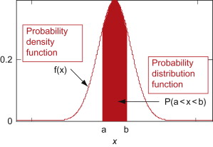
The probability distribution function is the integral of the probability density function. This function is very useful because it tells us about the probability of an event that will occur in a given interval.
Gamma distribution
The gamma distribution term is mostly used as a distribution which is defined as two parameters – shape parameter and inverse scale parameter, having continuous probability distributions. It is related to the normal distribution, exponential distribution, chi-squared distribution and Erlang distribution. ‘Γ’ denotes the gamma function.
Chi-square distribution
A random variable has a Chi-square distribution if it can be written as a sum of squares of independent standard normal variables. The Chi-square distribution is a theoretical distribution of values for a population.
Frequency factor method
Chow’s hydrological frequency factor, K, is used to compare and relate results and attach probabilities to several sets of maximum rainfall data. K is primarily a function of the recurrence interval for a particular probability distribution. K is displayed as a function of the mean of the annual maxima for both official and unofficial rainfall observations and the probable maximum precipitation (PMP) and PMP/2 for the 6 and 24 h durations.
Kuhn-Tucker conditions
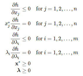
Kuhn–Tucker conditions, are first derivative tests (sometimes called first-order necessary conditions) for a solution in nonlinear programming to be optimal, provided that some regularity conditions are satisfied. Allowing inequality constraints, the KKT approach to nonlinear programming generalises the method of Lagrange multipliers, which allows only equality constraints.
KKT conditions is the necessary conditions for optimality in general constrained problem.
For a given nonlinear programming problem:
x* must satisfy all the following KKT conditions:
Simplex method
The Simplex method is an approach to solving linear programming models
by hand using slack variables, tableaus, and pivot variables as a means to
finding the optimal solution of an optimization problem.
A linear program is a method of achieving the
best outcome given a maximum or minimum equation with linear constraints.
To solve a linear programming model using the Simplex method, the following steps are necessary:
- Standard form
- Introducing slack variables
- Creating the tableau
- Pivot variables
- Creating a new tableau
- Checking for optimality
- Identify optimal values
The algorithm for linear programming simplex method is provided below:
- Establish a given problem. (i.e.,) write the inequality constraints and objective function.
- Convert the given inequalities to equations by adding the slack variable to each inequality expression.
- Create the initial simplex tableau. Write the objective function at the bottom row. Here, each inequality constraint appears in its own row. Now, we can represent the problem in the form of an augmented matrix, which is called the initial simplex tableau.
- Identify the greatest negative entry in the bottom row, which helps to identify the pivot column. The greatest negative entry in the bottom row defines the largest coefficient in the objective function, which will help us to increase the value of the objective function as fast as possible.
- Compute the quotients. To calculate the quotient, we need to divide the entries in the far right column by the entries in the first column, excluding the bottom row. The smallest quotient identifies the row. The row identified in this step and the element identified in the step will be taken as the pivot element.
- Carry out pivoting to make all other entries in column is zero.
- If there are no negative entries in the bottom row, end the process. Otherwise, start from step 4.
- Finally, determine the solution associated with the final simplex tableau.
Benefit-cost ratio method
- The benefit-cost ratio (BCR) is a ratio used in a cost-benefit analysis to summarize the overall relationship between the relative costs and benefits of a proposed project.
- If a project has a BCR greater than 1.0, the project is expected to deliver a positive net present value to a firm and its investors.
- If a project's BCR is less than 1.0, the project's costs outweigh the benefits, and it should not be considered.
- The BCR is calculated by dividing the proposed total cash benefit of a project by the proposed total cash cost of the project.
Linear programming
- Linear programming is a method of optimizing operations with some constraints. The main objective of linear programming is to maximize or minimize the numerical value.
- Linear programming is considered an important technique that is used to find the optimum resource utilization.
- Linear programming is the method of considering different inequalities relevant to a situation and calculating the best value that is required to be obtained in those conditions.
- The linear programming problem can be solved using different methods, such as the graphical method, simplex method, or by using tools such as R, open solver etc.
- The graphical method is used to optimize the two-variable linear programming. If the problem has two decision variables, a graphical method is the best method to find the optimal solution. In this method, the set of inequalities are subjected to constraints. Then the inequalities are plotted in the XY plane. Once, all the inequalities are plotted in the XY graph, the intersecting region will help to decide the feasible region. The feasible region will provide the optimal solution, as well as explains what all values our model can take. Let us see an example here and understand the concept of linear programming in a better way.
Reservoir routing
In Reservoir routing, the effect of a flood wave entering a reservoir is studied. Knowing the volume-elevation characteristic of the reservoir and the outflow-elevation relationship for the spillways and other outlet structures in the reservoir, the effect of a flood wave entering the reservoir is studied to predict the variations of reservoir elevation and outflow discharge with time.
This form of reservoir routing is essential
- in the design of the capacity of spillways and other reservoir outlet structures, and
- in the location and sizing of the capacity of reservoirs to meet specific requirements.
A variety of routing methods are available, and they can be broadly classified into two categories as:
- hydrologic routing, and
- hydraulic routing.
Hydrologic-routing methods employ essentially the equation of continuity.
Hydraulic methods, on the other hand, employ the continuity equation together with the equation of motion of unsteady flow. The basic differential equations used in the hydraulic routing, known as St. Venant equations, afford a better description of unsteady flow than hydrologic methods.
---
- The study material for AMIE/B Tech/Junior Engineer exams is available at https://amiestudycircle.com
- If you like the post please share your thoughts in the comment section


Comments